
- By R. Russell Rhinehart and Luis J. Yebra
- September 04, 2025
- Feature
Summary
Using variable speed drives on pumps reduces parasitic energy loss, enables proper maintenance and lowers capital costs.
This article examines a method for determining the optimal number and speed of parallel pumps to operate in response to flow rate and head demands. Although motivated by a parabolic trough solar-to-thermal power generation facility—an environmentally friendly energy source—the procedure seems applicable to many processes that use parallel pumps or blowers: water distribution, exhaust fans, etc.
The use of several parallel, smaller fluid-moving units instead of one large unit increases the reliability of on-stream time and optimizing the number of operating units reduces power consumption, wear, keeps spares available for maintenance or failures and increases the chance to use off-the-shelf (lower-cost) items. Although flow rate can be controlled by throttling valves with fixed speed pump drives, using variable speed drives to adjust the flow rate has considerable energy savings. Many readers will have applications with similar characteristics and may benefit from seeing this as a solution.
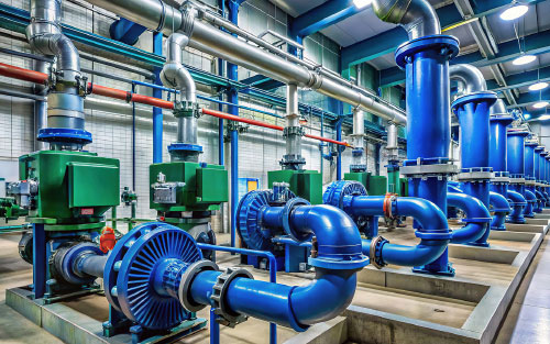
The Plataforma Solar de Almeria (PSA-CIEMAT) is a full-scale research center in southern Spain exploring approaches to generate electricity from thermal collection of solar energy. One of the facilities in research projects MODIAG-PTC (TED2021-129189B-C21/TED2021-129189B-C22) and DISOPED (PCI2022-134974-2) is the TCP-100 parabolic trough collector (PTC) (Figure 1). In PTC plants, the mirrors focus solar energy on a collection line through which thermal fluid (oil) runs and is heated to about 400 degrees C (752 degrees F), which makes steam to run turbo generators. The largest industrial PTC facilities in the world operate in the U.S (Mojave Solar Project and Solana Generating Station) generate 280 MW of electrical power and have more than 100 parallel collection lines. As the sun rises then sets and disturbances come and go, the required oil flow rate changes by about a 3:1 ratio and the system head requirement changes by about a 9:1 ratio. One challenge is to minimize pumping energy as solar irradiance and other conditions vary throughout the day.

Although the TCP-100 facility has three collection lines and one variable speed oil pump, this simulation study has 15 lines and five parallel pumps to preview complexity of the facility scale-up, a study that reveals the procedure. For other applications, the number of pumps and lines would depend on the technical and economic aspects of the project.
Figure 2 shows a representation of a PTC facility based on the TCP-100 plant design scale-up. There are ambient losses in each line, and for many reasons, the optical efficiency of each line is unique and changes over time. Oil from all lines is collected and fed to a boiler to produce steam. The variable speed pumps send cooled oil to the supply header for the solar collection lines. Throttling valves in the lines adjust the flow rate to make the exit temperature match a target. A reservoir provides oil thermal expansion, degassing and pump net positive suction head (NPSH) requirements.

The collection lines have individual efficiency factors. In addition, if covering a broad land area, irradiance on each line may be affected by local cloud shadows, mirror differences or such. This means that even if the flow rates through the lines are identical, the outlet temperatures may vary, but the mixed fluid must have the target temperature to operate the boiler. However, there is an upper temperature limit for the thermal fluid (typically about 400 degrees C [752 degrees F]).
To minimize pump energy consumption, the valve in the most efficient line is kept fully open and valves in the other N — 1 lines are adjusted to meet the temperature target in their outlets. The variable speed drives of the pumps are adjusted to keep the temperature of the most efficient line at target while providing the flow required by the other lines. There are M number of pumps, but only m are scheduled to be operating at any time instant with the objective of meeting flow-rate-head requirements near their most efficient operating point. In unconstrained operation, there are N + 1 decision variables: the number of pumps operating, pump speed and N — 1 valve positions.
In this study it is assumed that each of the five pumps are like the Dickow 65/320 pump of the TCP-100 facility, which has a 3:1 speed turndown ratio. The control valves in the lines have an equal-percent characteristic with a rangeability factor of 50 and electromechanical actuators. The lines have a seven cm diameter and a two-pass arrangement of 96 m each pass.
Models
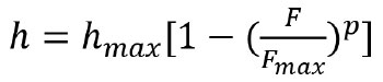
For this application, pump operating curves are very well matched with Formula 1a:
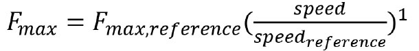
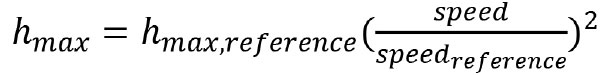
The classic similarity laws determine how the maximum flow rate and head scale with speed (Formulas 1b and 1c):
The coefficient values are shown in Table 1.
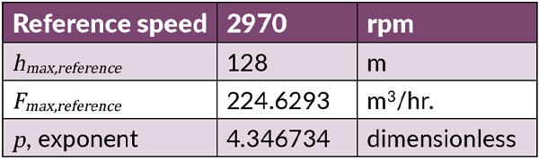
Table 1: Coefficient values.
Figure 3 shows the characteristic curves.

Pump efficiency curves are very well matched with Formula 2:
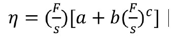
Where ![]() is in m3/hr. and
is in m3/hr. and ![]() is in rpm.
is in rpm.
The coefficient values are shown in Table 2.

Table 2: Coefficient values.
Figure 4 reveals how pump and drive overall power efficiency depends on flow rate and speed.

Although many use quadratic models (p = 2 and c = 1) as generic and mathematically convenient, the power law models provide improved fits to the manufacturer’s data. Users should find the model coefficients that best fit your pump/blower application.
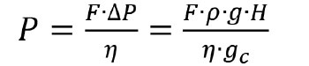
Given operational requirements (F & H), Equation Set (1) can solve for pump speed using root-finding algorithms, and then Equation (2) will provide the efficiency. Power consumed by the pump is then calculated as shown in Formula 3.
Control
Model-based control of the collection line temperatures (Rhinehart, R. R., Nonlinear Model-Based Control: Using First-Principles Models in Process Control, International Society of Automation, Durham, North Carolina, 2024, ISBN 13:978-1-64331-242-2) uses online data to calibrate optical efficiency and fluid pressure loss factors. The models then determine the required flow rate through each collection line. This gives the total flow requirement for the parallel pumps and also head losses within the boiler and recycle sections. With the valve on the most efficient line fully open, the collection line pressure drop is calculated, which provides the pressure drop for each of the lines, which is used to set valve positions to obtain target flow rates on the remainder N – 1 lines. The combined pressure drops provide the total head requirement. Then the number of pumps, m, simultaneously operating and their pump speed are optimized to minimize parasitic power losses.
Variable speed drive versus throttling
It is relatively simple to show the benefit of variable speed drives over throttling to adjust flow rate. With an initial condition of F = 150 m3/hr and H = 50 m, the scaled speed obtained is 0.82, the pump efficiency is 0.43, and the power is 37.6 kW. The new objective is to obtain the new flow rate of F = 50 m3/hr. By keeping the pump speed unchanged (having a fixed speed drive) and throttling the valve to increase H to 85 m, the flow rate is on target, and power drops to 19.7 kW. The main reason for the power reduction is the 1/3 reduction in F, but this is helped by a small improvement in efficiency, and it is countered by the increase in Head. See the middle rows in Table 3. But if flow is not throttled, and the head requirement is dominated by system friction losses (dynamic head) then the head requirement drops to 10 m. As the last row of Table 1 indicates, the pump speed can be reduced further, with a substantial improvement in power to 2.1 kW, representing about a 90 percent reduction compared to throttling.
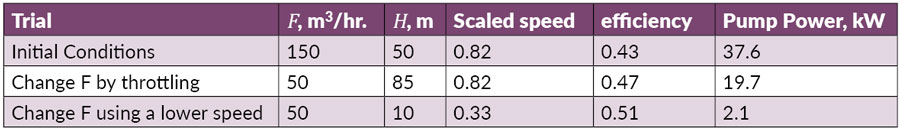
Table 3: A comparison of throttling and speed reduction.
Process pump optimization
With pumps in parallel, the number of active pumps at any moment can be chosen to minimize pumping energy. Nominally, if there are m number of operating pumps, each will have 1/mth of the total required flow capacity and the same head required to drive the total fluid through the entire piping system.
For each possible choice of the number of active pumps calculate the pump speed to make the pump model match
  and
and  . If the number of pumps is too few, then the speed, s, will be in excess of the maximum. If m is too large, then the speed will fall below the minimum. For valid m choices, calculate efficiency, then determine the total power required. Then, choose the feasible number of operating pumps that results in the minimum power.
Results
Figure 5 reveals how solar irradiance, normal to the aimed mirrors, changes during an 8-hr. operating period. At about 1:30 PM the irradiance drops by about 50 percent simulating an hour of cloud cover. The horizontal line represents the mixed oil temperature (all individual lines are within a tenth of a degree Centigrade of the setpoint). The control scheme keeps the temperature of each line at the setpoint of 395 degrees C (743 degrees F), except for a brief mid-day period that strains pump capacity, elevating the temperature by less than 1 degree C (33.8 degrees F), and a switching disruption that lowers the temperature by a few tenths of a degree Centigrade.

Figure 6 reveals how the total flow rate (red), optimum number of pumps (blue) and per pump flow rate (gray) change with time.

For most of the day (irradiance less than 1,000 W/m2), optimization determines that only one of the five pumps should operate. Oil flow rate is nearly proportional to the irradiance, and pressure drop is roughly proportional to the square of flow rate (the square of irradiance), as a result the power required to drive the fluid is roughly proportional to the cube of irradiance, ![]() , which rapidly drops after reaching the peak irradiance of 1,100 W/m2.
, which rapidly drops after reaching the peak irradiance of 1,100 W/m2.
Figure 7 reveals how pump speed and valve positions change with time due to irradiance. The relatively horizontal lines at the top of the graph are valve positions. They trace a symmetrical path as the sun is rising or falling. The top line is Valve 1—the most optically efficient line—which stays fully open.
The blue curve represents the pump speeds, which are limited to 1,000 and 2,970 rpm. The discontinuities in speed are due to changing the number of pumps. The small speed discontinuities at about 11:30 a.m. and 12:30 p.m. are barely noticeable.

The power savings of the optimum number of pumps relative to running all five is shown in Figure 8.

This indicates a 3.4% savings in pump power for about half the day, because the m pumps are operating close to their optimum efficiency.
Reducing the number of pumps when they are not all needed means that operational wear on pumps can be lessened by running fewer when not all are required. In addition, this strategy has pumps running near the best efficiency point (BEP) and keeps the pumps operating in their preferred operating range. These are important ancillary benefits to the parasitic power reduction.
Wrapping up
Using variable speed drives and optimizing the number of operating pumps has a significant impact on parasitic energy losses. It also benefits maintenance. And, system design using several smaller standard sized pumps, instead of one special pump, provides capital cost savings and reliability advantages.
This feature originally appeared in the August/September issue of Automation.com Monthly.
About The Author
R. Russell Rhinehart is a professor emeritus at Oklahoma State University, Stillwater, Okla.
Luis J. Yebra is a researcher at CIEMAT research center, Plataforma Solar de Almeria (PSA-CIEMAT), in Almeria, Spain. This full-scale research center investigates approaches for generating electricity from the thermal collection of solar energy. The TCP-100 parabolic trough collector (PTC) referenced here is one of the facilities in research projects MODIAG-PTC (TED2021-129189B-C21/TED2021-129189B-C22) and DISOPED (PCI2022-134974-2).
Did you enjoy this great article?
Check out our free e-newsletters to read more great articles..
Subscribe