
The following discussion is part of an ongoing column called Ask the Automation Pros, authored by Greg McMillan, 2010 ISA Life Achievement Award recipient, industry consultant and author of numerous process control books and articles. Submit your questions to [email protected] with “Ask the Automation Pros” in the subject line. Browse previous questions and answers here. Past Q&A videos are also available on the ISA YouTube channel; you can view the playlist here.
Erik Cornelsen’s question
In a simple proportional-integral-derivative (PID) loop (single control variable, single manipulated variable) where rapid or slow manipulated variable changes are needed in one direction or both directions, what is the best strategy to get the best rate of change in the controller output? What are some examples of applications where this is important? Is adding a ramp or a rate limiter function block after the PID output the correct approach, or is there a more elegant solution within the control strategy itself? Please provide some guidance on how PID tuning can meet objectives. How should start-up, product transition, abnormal operation and shutdown phases be handled in situations where the manipulated variable needs to experience large, rapid changes?
George Buckbee’s response
I have seen many scenarios over the years, including:
- A desire to reduce the travel on a very large, expensive, remotely operated valve
- The need to reduce sudden draws on a header that would upset header pressure and affect other users
- Batch-driven steam loads, where upstream supply needs time to ramp-up/respond versus tripping the boiler
- Desire to reduce overshoot
- Setpoint ramping, because the user wants the loop tuned for fast disturbance rejection, but does not need to trigger sudden movement when adjusting the setpoint
Pat Dixon’s response
It begins with recognizing the objective of the loop. Erik has already done this, but so many assume that every loop is the same and try to tune tightly. The ISA 5.9 technical report explains this very well.
To minimize rapid manipulated variable changes, I prefer to do this with tuning as much as possible. This means no derivative and little, if any, proportional control. Adding a ramp or rate limiters to the output can create a mismatch between tuning and the output response. Another approach is to filter the input so that when there is a step change in the process variable, the loop responds to a smooth input, which reduces the output rate of change. I think applying filtering to the input is better than rate limiting the output because it makes loop tuning match the filtered input and is more intuitive to maintain.
I also think using a gap can be helpful if you are trying to minimize output moves in a process exhibiting negligible change (steady state).
For start-up and shutdown, I have successfully implemented sequences that ramp an output during those phases and put the controller in auto when process reaches a steady state.
Here are a couple of things to consider regarding start-up/shutdown:
- If it is important to control the process variable during start-up/shutdown, setpoint ramping can help. This is a common feature in control systems that makes it easy to specify the target setpoint and the time or rate for getting there.
- A caveat is that start-up or shutdown conditions may represent significantly different process responses. Nonlinear gain could be addressed with gain scheduling, but the dynamics can be different if liquid volumes are smaller than during steady state operation. It is possible that closed-loop control might not be possible in this transition. A sequence that ramps the output during the transition and returns it to closed-loop control in auto when the process reaches a steady state can be a good approach in this case.
Greg McMillan’s response
It is first important that the measurement type and installation minimize noise. For example, the straight runs and sizing of differential head and vortex meters are critical, and magmeters and Coriolis meters offer a much more accurate, lower noise signal, especially at low flows. Temperature sensors in tapered thermowells with good insertion lengths in well-mixed zones free from bubbles with head-mounted transmitters offer the best accuracy and least noise. Signal filters should be judiciously applied to reduce noise to keep output changes within control valve resolution limits. The filter time should be less than 20% of the reset time to prevent increasing the integrated error practical limit by more than 20% and less than 20% of the dead time to prevent increasing the peak error ultimate limit by 20% for lag dominant processes, as detailed in ISA-TR5.9-2023, Section 7. The derivative filter built into PID algorithms may be adjustable and intelligently adaptable.
While proportional action causes more sudden changes in controller output, it is critical to realize that it has a sense of direction, unlike integral action, and is satisfied for a resting process variable. Also, the peak error for load upsets and the rise time for setpoint changes are inversely proportional to the PID gain. The remaining error for proportional-only controllers is inversely proportional to the PID gain. For temperature control of runaway processes, high PID gain and rate settings and minimal integral action are used to ensure safe operation. Integral action has no sense of direction and will be driving the controller in the wrong direction as a process variable is approaching the setpoint. Also, integral action is never satisfied and will continue to change output even when the error is negligible. Integral action at one or more points in the loop causes limit cycles from resolution limits (stiction). Integral action at two or more points in the loop causes limit cycles from lost motion (backlash). See ISA-TR75.25.02-2024, Annex A, for more details on how tuning affects limit cycles. Shinskey advocates proportional-only control for level and secondary loops. I advocate proportional-only control in positioners to enable using higher positioner gain settings and to reduce and eliminate limit cycles.
In near-integrating, true integrating and, particularly, runaway processes, proportional action is critical for safety. Users like integral action because they are focused on the process variable error and not the process variable change direction, and the action is more gradual. James Beall and I have found that in many vessel temperature and pressure loops, the reset action used is 10 to 100 times larger than what is best. However, in flow loops and loops with small process time constants, especially dead time dominant loops, proportional action needs to take a back seat to integral action. Lambda tuning for self-regulating processes takes this into account and then makes a transition to integrating process tuning for lag dominant processes classified as near-integrating processes.
There are several examples noted in ISA-TR5.9-2023, Section 6.6, on the need for PID directional move suppression (DMS), a stand key feature of model predictive control and the use of external reset feedback (ERFB) (Section 7.4.3) action to enable DMS by the simple use of PID output rate limits without PID tuning issues. The classic DMS case is compressor surge control, where a slow approach to better energy use and fast getaway for surge protection. DMS provides a more accurate, sustainable and maintainable solution than is traditionally done by a fast-opening and slow-closing surge valve that posed tuning problems and the difficulty in the setting and maintenance of the different stroking rates. A similar DMS approach is used for Resource Conservation and Recovery Act (RCRA) pH control to conserve reagent usage, where a fast-opening and slow-closing reagent valve is needed. DMS is helpful for fast-opening and slow-closing coolant valves for runaway reactor temperature control. There is also a general need to slow down the reversal of PID controller output to prevent an unnecessary crossing of the split range point where stiction is greatest causing limit cycles. For valve position and override controllers, a slow approach to the optimum and fast getaway for upsets is best achieved by DMS with ERFB.
For start-up, transitions, changes and shutdowns, fast changes via setpoint feedforward and procedure automation (ISA-TR5.9-2023, Section 7.4.8) are useful.
Russ Rhinehart’s response
That is an interesting question. Is an integral-only controller, or one with very low proportional gain, a solution to slow down the manipulated variable rate of change?
I think the rate-limiting function on the controller output will also work, but it is an override. Therefore, I recommend using external reset feedback for the controller bias adjustment instead of the integral method.
If a fast manipulated variable response is desired for start-up and shutdown, and a tempered manipulated variable response is desired only for regulatory periods, then a solution may be to switch tuning for the separate conditions.
Do you want to set up the controller within a structure so that people who might want to tune it online cannot make it aggressive? If you add rate limiting to the output, then those trying to tune the controller will be frustrated with the constrained controller behavior.
I’m just reading in the question the phrase “where rapid or slow manipulated variable changes are needed in one direction or both directions.” A possible solution is a cross-limiting strategy, such as that used in burner control, where increasing fire increases air flow first, then fuel follows, but decreasing fire decreases fuel first, then air follows. This ensures that there is always excess oxygen in the flue gas.
Michael Taube’s response
First, the terms “fast,” “slow” and “sudden” change are quite subjective, so we need better definitions.
Second, what is the source of the process “sensitivity” to “rapid changes”? Is this a reaction kinetics issue, (highly) nonlinear behavior or other issue, and can we model it reasonably accurately?
Third, what is the primary control (operational) objective, as well as secondary, tertiary and other levels of concern? How are these objectives affected by the operational phase (i.e., start-up, shutdown, “steady state,” etc.)? To be clear, the control objective(s) should help, support and aid the operator in achieving the operational objective(s); that’s why I phrase it as such. If the control objective isn’t aligned with the operational objective, then the control design is wrong. It is usually assumed that they are aligned, thus it’s rarely questioned. It is vital, however, that the assumption be validated during the design process.
Now to the point: PID control is wildly flexible, albeit fixed (once “tuned”), in its potential response to setpoint changes and unmeasured disturbance rejection without the need for ramps, (output) filters and/or other “functional appendages” (with certain exceptions—details to follow). One of the first items to acknowledge is that PID is, in fact, a model-based controller that is contingent on:
- The process behavior model(s): This includes process gain, dominate lag and dead time, as well as, perhaps, a second lag and/or lead time (the last two are only rarely needed to provide a suitably accurate process model). It is an integrating process versus an open-loop, stable process. Also, if the process behavior changes depending on its current operational phase, run time and/or other parameters/conditions, then this, too, must be taken into account in the process model, including nonlinear steady-state behavior.
- The controller response model(s): This is the model for how the controller is to respond to setpoint changes and disturbances (i.e., quarter amplitude decay, over-damped, under-damped and other changes).
- The PID structure: It is critical to know the PID structure (e.g., ideal, parallel, interactive), whether a process variable or error is used by proportional or derivative actions, values for any internal filters (such as the signal filter for the derivative action), and the controller’s execution period (or execution rate) relative to the process’s dynamic behavior.
“Tuning Rules” take all of the above into account and generate the PID tuning parameters for a given process model. Thus, if the process model is reasonably accurate, and the PID form/structure is also known, then one can begin to develop the tuning rules that produce the desired response (if existing tuning rules are deemed unsuitable).
Where might “functional appendages” be required? If the process behavior (model) changes significantly and/or the required controller response (model) to setpoint changes/disturbances must differ across the process’s operating envelope, then this is where additional functionality or “enhancements” may be required. Many control systems provide a variety of optional features for the PID function (and input/output processing), including:
- “Error-squared” algorithm: This makes the proportional response more aggressive the further away the process variable is from the setpoint.
- Output/valve characterization: This very useful feature accounts for “simple,” nonlinear flow behavior.
- Dynamic tuning parameter updating: Often a “roll-your-own” situation for the (rare?) case where the process behavior changes significantly over the operating range.
While PID tuning can be updated dynamically based on the current operating point, other physical enhancements may also be required, such as different-sized control valves (flows) for coarse versus fine adjustments (e.g., pH control). This is where solid process understanding comes into the design of the controls and tuning: a “simple” single-input, single-output controller may not suffice, even if only one PID function block is used for the control loop.
Russ alluded to another vital aspect of any implementation: Ongoing support and maintenance by someone other than the original control designer. This is where one of my favorite topics comes into play: documentation. The designer(s) must provide detailed documentation of the final implementation, as well as the basis for the process and controller models, any known (or suspected) limitations, the considerations that drove the design (e.g., why this design versus other possible ones) and/or possible future enhancements. Pat also makes a great point regarding the use of process variable filters versus output rate clamps. I’ve seen some really wild tuning “lobotomized” by output rate clamps. It took quite a while for me to figure out why changing the tuning didn’t affect the controller behavior because the output clamping (which is an offered but rarely used feature on many control systems) was displayed on a different tab or section of the PID function block (a separate tab where the tuning parameters are displayed).
Short version: Don’t use output rate clamps to cover up tuning problems. Finally, Greg McMillan has several books on pH and compressor control that address implementing “variable response” control for these types of issues. Also, a great paper — “A Plant-wide Industrial Process Control Problem” published in Computers Chemical Engineering, Vol. 17. No. 3, 1993, detailing an example in the “The Tennessee Eastman Challenge Problem (TECP)” dynamic modeling initiative — by J.J. Downs and E.F. Vogel looks at a generalized nonlinear exothermic reactor control problem that illustrates the challenges in implementing control, of any variety, on “sensitive” processes. My academic colleagues, Isuru Udugama and Christoph Bayer (TH-Nürnberg), used the TECP in undergraduate process control courses to illustrate the importance of robust controls design and had very positive feedback from the students.
Michel Ruel’s response
1. Tune to the control objective. Adjust the loop tuning to meet the intended control goal. As part of tuning, choose the appropriate filtering to remove high‑frequency noise that the PID cannot handle. As a rule of thumb, the filter time constant should be a fraction of the loop response (closed‑loop time constant) and the process dead time. For loops tuned tightly for disturbance rejection, use a filter time constant of roughly one-fifth of the process dead time (see ISA technical report ISA-TR5.9-2023).
2. Use adaptive or split‑range tuning when needed. If the control objective differs for small versus large errors, consider adaptive tuning or a PID with different parameter sets (or a PID gap). Tuning can be changed based on conditions (start‑up, normal, excessive error and shut‑down), on the magnitude of the error, or on another relevant process variable. For large setpoint changes, consider a PID with two degrees of freedom (2 DOF) or apply a setpoint filter.
3. Avoid restrictive limiters on the PID. Avoid using ramp limiters or “shackles” directly on the process variable, setpoint or controller output (CO) whenever possible—these introduce nonlinearity and can degrade performance. A properly tuned PID controller rarely needs such limits.
4. Review adjacent loops. A loop rarely operates alone. Excessive tuning changes (adapting tuning) might be reduced by reviewing and coordinating the tuning of neighboring loops to match overall process objectives.
Erik Cornelsen’s response
Thank you all for the very interesting points highlighted in the document.
I just wanted to clarify something regarding Michel’s Point 1, specifically the recommendation under “Tune to the control objective” about using a filter time constant of roughly one-fifth of the process dead time.
Is the recommendation to apply a filter within the PID block to the derivative term, like a delay of the derivative action? If so, how would this apply in cases where the controller is configured as PI only, without a derivative term or where the PID block does not offer a derivative lag function?
In those situations, would applying a filter to the process variable input signal achieve a comparable result? If yes, which type of filter would be the most appropriate, for example, a moving average or a first-order lag filter?
Michel Ruel’s response
The suggested filter is for the process variable (hence the error sent to PID will be filtered) to reduce the noise (noise corresponds to fast disturbances, too fast for the PID to handle). Reducing the noise will reduce the valve movements.
If the loop is tuned for disturbance rejection, the control loop response time will be 6 to 10 times the apparent dead time. Using a first-order filter time constant that is too large will slow down the loop and require reducing the proportional gain. Using a first-order time constant that is too small will let too much noise go through the controller. Using a filter time constant of a fraction of the dead time corresponds to a good balance; I usually suggest one-fifth of the apparent dead time.
We usually configure a first-order filter (some systems offer a second-order, usually a Butterworth, filter) and avoid a moving average (a nonlinear function such as a ramp) except for special cases.
The filter for the derivative is different; it is used only to filter the signal going to the derivative function. This derivative filter is essential to avoid high noise at the derivative function output.
Peter Morgan’s response
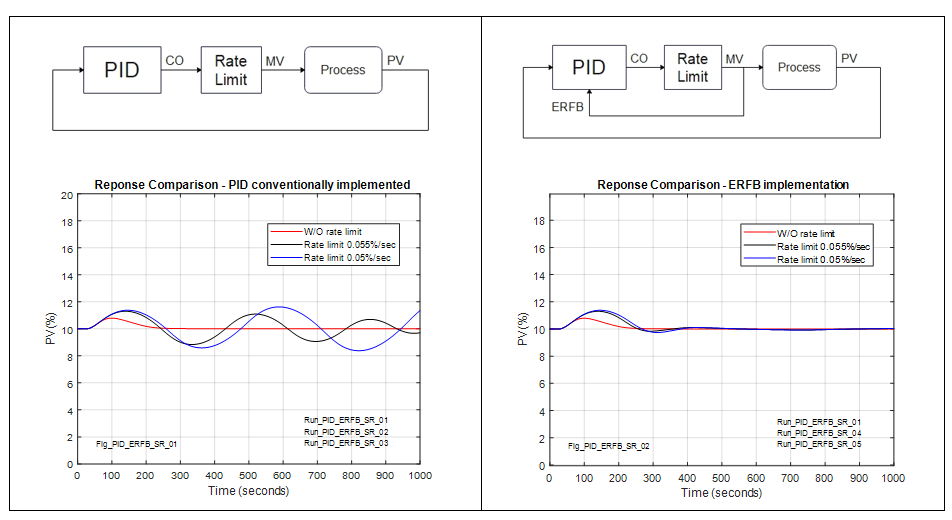
Without prejudice to the advice given here against the use of rate limits to moderate controller action, I could not resist this opportunity to demonstrate the benefits of a PID implementation using filtered positive feedback to take advantage of ERFB for response improvement. Later, I provide my own cautions regarding the use of rate limits.
When a rate limit is added at the PID output for a conventionally implemented PID and the rate limit is active, the integral term accumulates without an effect on the manipulated variable or process variable. When there is finally a correction in the process variable that requires the controller to reverse the action on the manipulated variable, the integral term must unwind, introducing latency in the action, causing overshoot and reducing stability. Readers comfortable viewing the effect in the frequency domain might draw the conclusion that adding the rate limit introduces a phase shift when it is active. In the plot for the conventional PID, for a 5% load disturbance with the rate limit added to the controller set to 100%/s and of little effect, and an actuator rate limit (in the modeled process) of 20%/s, the response is without overshoot, settling in 200 s (approximately). When the rate limit at the controller is reduced to 0.05%/s (slew time = 10 times the dominant process time constant), the response is highly oscillatory and ultimately winds up in a limit cycle.
When the integral action is implemented using filtered positive feedback, the feedback is derived from the output of the rate limit as external reset feedback and the rate limit is active, the positive feedback cannot rise above the rate-limited value for an increasing output and cannot fall below the rate-limited value for a reducing output. In this way, the accumulation occurring with the conventionally implemented PID algorithm is avoided, and the latency in action on an error reversal is avoided.
Comparing the response on the right plot with that on the left vividly demonstrates the improvement in response when ERFB is implemented. Of course, if the rate limit is in play for a load change, the peak change in the process variable will be higher, that is, without the rate limit. It should be noted that, but for the use of ERFB, the control parameters are the same for both cases.
Notwithstanding that there may be good reasons for not adding a rate limit at the output of the PID, if a rate limit is required because of certain operating conditions or identified restrictions on loading rates on the process, a PID implementation allowing ERFB should be considered. Note that some, but not all, Distributed Control System (DCS) vendors offer ERFB as a configurable option, and for those that do offer it, the implementation should be verified.
 Before adding a rate limit, the adjustment of controller tuning parameters should be considered as a means of meeting any loading restrictions that might apply. A controller implementing 2 DOF might offer a solution that provides the performance required for setpoint and load changes without violating loading restrictions. Restricting the proportional action so that it acts only on the change in the process variable or the weighted change in the setpoint and configuring the derivative term so that it acts only on the process variable are options for tailoring the response of the loop to balance response targets and process loading restrictions.
Cautions when adding a rate limit. When the output of a non-initializable rate limiter connects to the analog output, a controller download may require the mode of the field element or local system to be placed in manual or local control to avoid an upset. When the rate limit output is forwarded to an auto/manual station, for bumpless transfer of the downstream loop to auto or cascade (depending on strategy), the rate limit must be initialized to match the downstream loading/demand.
Because it is common that the auto/manual station for the controller is integral with the PID function, inserting a rate limiter after the PID will require an informed decision as to whether the rate limit should apply in manual as well as auto. Furthermore, because the panel operator rightly expects the final element to hold its last position when the controller is initially transferred to manual, the manual position demand should momentarily align with the rate limit output before the controller is released to manual.
For start-up and shutdown. Several times (maybe more than I remember), I have used a little logic with a ramp function for start-up and shutdown sequencing. In strategies where the demand is ordinarily determined by a PID controller, when the sequence is not active and the ramp output is not selected, the ramp output should follow the demand from the controller so that the demand in the start-up or shutdown mode starts from the last controller output, that is, without disturbance or latency. Similarly, when the start-up or shutdown sequence is active, the controller output should follow the ramp output so that when the sequence terminates and the controller output is selected, adjustment can continue under the action of the controller without disturbance. Most vendors make provisions for output tracking at the PID controller that allow strategies of this kind to be implemented.
I recommend these resources for those interested in learning more about ERFB:
- “The power of external reset feedback” by F. G. Shinskey.
- “Deadtime compensation opportunities and realities” by Peter Morgan and Greg McMillan. Note that any search for information on ERFB will show that Greg McMillan has been a longtime proponent of ERFB.
- ISA Technical Report ISA-TR5.9-2023, Proportional-Integral-Derivative (PID) Algorithms and Performance.
Beb Heider’s response
Russ’s last comment made me think of a strategy I used once for batch weighing called “a derivative controlled low-pass filter,” where high frequency noise increased filtering and a step change decreased filtering. This is detailed on pages 222-225 of Daniel H. Sheingold’s Transducer Interface Handbook – A Guide to Analog Signal Conditioning.
About the authors
- Erik Cornelsen
- George Buckbee
- Michael Taube
- Pat Dixon
- Gregory K. McMillan
- Russell Rhinehart
- Michel Ruel
- Peter Morgan
- Bob Heider
Further reading
- Downs, J.J. and Vogel, E.F. “A Plant-wide Industrial Process Control Problem,” Computers Chemical Engineering, Vol. 17. No. 3, 1993. https://www.abo.fi/~khaggblo/RS/Downs.pdf
- ISA-TR5.9-2023. Proportional-Integral-Derivative (PID) Algorithms and Performance. International Society of Automation. https://www.isa.org/products/isa-tr5-9-2023-proportional-integral-derivative-pi
- ISA-TR75.25.02-2024. Test Procedure for Control Valve Response Measurement from Step Inputs. International Society of Automation. https://www.isa.org/products/ansi-isa-75-25-01-2024-test-procedure-for-control
- Morgan, Peter and Greg McMillan. “Deadtime compensation opportunities and realities.” Control, 2024. https://www.controlglobal.com/control/loop-control/article/55090399/deadtime-compensation-opportunities-and-realities
- Sheingold, Daniel H. Transducer Interface Handbook – A Guide to Analog Signal Conditioning. Analog Devices, Inc., 1980.
- Shinskey, F. G. “The power of external reset feedback.” Control, 2006. https://www.controlglobal.com/control/plcs-pacs/article/11383110/process-automation-technologies-programmable-logic-controllers-the-power-of-external-reset-feedback-control-global